Modeling and Solving
Overview
minimize  2*(3*a+b)*b**2 + 3
s.t.      a*b >= 2
          0 <= a <= 1, a is integer
          1 <= b <= 2, b is continuous
This optimization problem is a kind of the mixed integer constrained non-linear programming. This problem can be formulated using flopt as follows.
import flopt

# variables
a = flopt.Variable(name="a", lowBound=0, upBound=1, cat="Integer")
b = flopt.Variable(name="b", lowBound=1, upBound=2, cat="Continuous")

# problem
prob = flopt.Problem(name="Test")

# set objective function
prob += 2*(3*a+b)*b**2+3

# set constraint
prob += a*b >= 2

# run solver
prob.solve(timelimit=0.5, msg=True)

# get best solution
print("obj value", prob.getObjectiveValue())
print("a", a.value())  # or flopt.Value(a)
print("b", b.value())
Variables
0 <= a <= 1, a is integer
1 <= b <= 2, b is continuous
In flopt, we denote these variables as
from flopt import Variable

a = Variable(name="a", lowBound=0, upBound=1, cat="Integer")    # is equal to Variable("a", 0, 1, flopt.VarInteger)
b = Variable(name="b", lowBound=1, upBound=2, cat="Continuous") # is equal to Variable("b", 1, 2, flopt.VarContinuous)
We can set an initial value to each variable by ini_value option. If no initial value is set, the initial value is randomly set from the possible values of the variable.
b = Variable("b", 1, 2, "Continuous", ini_value=1.5)
Note that duplicate variable names are discouraged and often cause unexpected behavior in the execution phase of the algorithm.
Flopt provides some variables categories.
# Integer (flopt.VarInteger) -- for variable takes only integer values
x = Variable("x", cat="Integer")

# Binary (flopt.VarBinary) -- for variable takes only 0 or 1
x = Variable("x", cat="Binary")

# Spin (flopt.VarSpin) -- for variable takes only -1 or 1
x = Variable("x", cat="Spin")

# Continuous (flopt.VarContinuous) -- for variable takes real numbers
x = Variable("x", cat="Continuous")

# Permutation (flopt.VarPermutation) -- for permutation variable
x = Variable("x", lowBound=0, upBound=5, cat="Permutation")
Permutation variable has a permutation. We use this variable to model the problem that optimizes the permutaion, sush as Travelling salesman problem or the quadratic assignment problem (QAP).
In addition, we can create multiple variables as array or dictionary format.
from flopt import Variable

#
# variables as array
#
Variable.array("x", 5)  # (name, shape)
>>> FloptNdArray([Variable("x_0", None, None, "Continuous", -7.298898175196169e+17),
>>>                Variable("x_1", None, None, "Continuous", 2.268338741196992e+17),
>>>                Variable("x_2", None, None, "Continuous", 6.223164001493279e+17),
>>>                Variable("x_3", None, None, "Continuous", 3.651409812719841e+17),
>>>                Variable("x_4", None, None, "Continuous", -7.981446809145265e+17)],
>>>                dtype=object)

Variable.array("x", (2, 2))  # (name, shape); this is equal to flopt.Variable.matrix("x", 2, 2)
>>>  FloptNdArray([[Variable("x_0_0", None, None, "Continuous", -1.1465787630314445e+17),
>>>                  Variable("x_0_1", None, None, "Continuous", -4.926156739107439e+17)],
>>>                 [Variable("x_1_0", None, None, "Continuous", 8.384051961545784e+17),
>>>                  Variable("x_1_1", None, None, "Continuous", -7.166609437648443e+17)]],
>>>                dtype=object)

#
# variables as dict
#
Variable.dict("x", range(2))  # (name, shape)
>>> {0: Variable("x_0", None, None, "Continuous", 7.270654090642355e+17),
     1: Variable("x_1", None, None, "Continuous", -1.180838388759273e+17)}

Variable.dict("x", (range(2), range(2)))  # (name, shape)
>>> {(0, 0): Variable("x_0_0", None, None, "Continuous", 8.675657447208325e+17),
     (0, 1): Variable("x_0_1", None, None, "Continuous", 6.122390620359232e+17),
     (1, 0): Variable("x_1_0", None, None, "Continuous", 6.323625756142303e+17),
     (1, 1): Variable("x_1_1", None, None, "Continuous", 6.91510665884983e+17)}

Variable.dicts("x", (range(2), range(2)))  # (name, shape)
>>> {0: {0: Variable("x_0", None, None, "Continuous", -7.478838052120259e+17),
         1: Variable("x_1", None, None, "Continuous", 9.81873816586668e+17)},
     1: {0: Variable("x_0", None, None, "Continuous", -5.518448165239538e+17),
         1: Variable("x_1", None, None, "Continuous", -7.32344708203296e+16)}}
Expression
We can represent expression from operation of variables and expression.
import flopt

x = flopt.Variable("x")
y = flopt.Variable("y")

z = x + y
z = x - y
z = x * y
z = x / y

w = z * (x ** z) / y
q = w ** z / z
Value of expression is calcluated by values of variables.
x = flopt.Variable("x", ini_value=1)
y = flopt.Variable("y", ini_value=2)
z = x + y
print(z.value())
>>> 3
In addition, flopt provides some mathematical operations.
x = flopt.Variable("x")

z = flopt.cos(x)
z = flopt.sin(x)
z = flopt.abs(x)
z = flopt.floor(x)
...
This mathematical operations affect array-like variables element by element.
x = flopt.Variable.array("x", 3)
>>> FloptNdarray([Variable("x_0", None, None, "Continuous", -61809393740223.375),
>>>               Variable("x_1", None, None, "Continuous", 636452077623562.0),
>>>               Variable("x_2", None, None, "Continuous", 65797807764902.125)],
>>>              dtype=object)

flopt.cos(x)
>>> FloptNdarray([Cos(x_0), Cos(x_1), Cos(x_2)], dtype=object)
We can represent the blackbox function as CustomExpression.
def user_defined_fn(a, b):
    return simulation(a, b)

x = flopt.Variable("x")
y = flopt.Variable("y")

z = flopt.CustomExpression(user_defined_fn, args=[x, y])
z.value()  # value calculated through user_defind_fn(x, y)
Problem
We can model optimization problem using Problem class of flopt. We set objective function and constraints into problem class object. The objective function and constraints are created by arithmetic operation of variables and expression.
Objective function
We set the object function to Problem using += operation or .setObjective function.
prob = flopt.Problem(name="Test", sense="Minimize")
prob += 2*(3*a+b)*b**2+3   # set the objective function
# prob.setObjective(2*(3*a+b)*b**2+3)   # same above
When we solve a maximize problem, we set sense=”Maximize” (default is sense=”Minimize”).
prob = flopt.Problem(name="Test", sense="Maximize") # is equal to sense=flopt.Maximize
Constraints
Constraint is created by ==, <= or >= of expression, variables or constant. We add the constraint into problem by += or .addConstraint().
prob += a*b >= 2
prob += a*b == 2
prob += a*b <= 2
The details of user’s defined problem can be shown by .show().
prob.show()
>>> Name: Test
>>>   Type         : Problem
>>>   sense        : Minimize
>>>   objective    : 2*((3*a+b)*(b^2))+3
>>>   #constraints : 1
>>>   #variables   : 2 (Continuous 2)
>>>
>>>   C 0, name None, 2-(a*b) <= 0
>>>
>>>   V 0, name b, Continuous 1 <= b <= 2
>>>   V 1, name a, Integer 0 <= a <= 1
Solve
We can obtain the solution of the problem by prob.solve(). If no solver argument is specified, an algorithm that can solve the problem is automatically selected by flopt. The user can limit the algorithm’s execution time by specifying timelimit. When timelimit is not set, note that this function is often time-consuming because it essentially runs until the algorithm satisfies the termination condition.
prob.solve(timelimit=0.5, msg=True)
Full minimul example code is here.
import flopt

a = Variable(name="a", lowBound=0, upBound=1, cat="Integer")
b = Variable(name="b", lowBound=1, upBound=2, cat="Continuous")

prob = flopt.Problem(name="Test", sense="Minimize")
prob += 2*(3*a+b)*b**2+3

# run solver
prob.solve(timelimit=0.5, msg=True)
Solver
When you want to select algorithm to solve problem, you create a Solver object and specify it as solver parameter in problem.solve().
import flopt

solver = flopt.Solver(algo="Random")  # select the heuristic algorithm
solver.setParams(timelimit=0.5)  # setting of the parameters
prob.solve(solver=solver, msg=True)  # run solver
Parameters specific to that algorithm are set using .setParams(name=value, …). If user has a dictionary d of keys are parameter names and values is their corresponding values, you can set the parameters together using .setParams(**d).
Users can use some third-party solvers and solvers implemented in flopt. flopt.Solver_list() shows all solvers available in flopt and flopt.allAvailableSolvers(problem) shows all available solvers for user defined problem.
import flopt

a = flopt.Variable("a", 0, 1, cat="Continuous")
b = flopt.Variable("b", 1, 2, cat="Continuous")

prob = flopt.Problem(name="Test")
prob += 2*a + 3*b
prob += a + b >= 1

flopt.allAvailableSolvers(prob)
>>> ['Pulp',
>>>  'Scipy',
>>>  'ScipyMilp',
>>>  'Cvxopt',
>>>  'auto']
You can specify the available solver by declaring solver object or specifing the solver name.
solver = flopt.Solver(algo="Scipy")
prob.solve(solver=solver)

# or
prob.solve(solver="Scipy")
AutoSolver
Flopt provides AutoSolver as a default solver. AutoSolver selects the appropriate solver for the user modeled problem.
solver = flopt.Solver(algo="auto")
When we check which solver is selected, we execute solver.select(prob).name.
solver = flopt.Solver(algo="auto")
solver.setParams(timelimit=1)
solver.select(prob).name
>>> 'ScipyMilp'
Result
The result of the solver is reflected in Problem and Variable objects.
getObjectiveValue() in problem shows the objective value of the best solution solver found.
.value(), flopt.value(), flopt.Value() shows the value of variable of the best solution.
print("obj value", prob.getObjectiveValue())
print("a", a.value())  # or flopt.Value(a)
print("b", b.value())
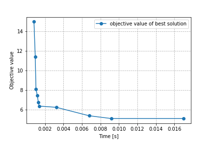
Solver Profiling
You can easily see the transition of the incumbent solution.
status, logs = prob.solve(solver, msg=True)  # run solver
fig, ax = logs.plot(label="objective value of best solution", marker="o")